
Application background
The data set chosen for this project contains the transactions of a UK-based online retailer occurred between 01/12/2009 and 09/12/2011.The items sold comprise a wide range of giftware and many customers are wholesalers. Source: UCI - Machine Learning Repository There are several reasons why we found this data set to be an ideal candidate for a market basket analysis:
- good number of available attributes, useful not just for association rule mining but potentially a variety of other techniques as well (eg. clustering, classification);
- large number of transactions (~1M);
- quality of the data (limited % of missing values).
Data Exploration
The dataset presented most of the columns filled with data, with only columns ‘Description’ and ‘Customer ID’ as missing values. However, the null Description cells only accounted for 0.41% of the whole column, meanwhile 22.77% of the Customer ID rows were empty. The null Description rows were removed, as the impact would be inconsequential. While the Customer ID rows remained for Data Exploration, as these rows held valid product information to help with customer behaviour analysis. However, was later removed for RFM Analysis and Clustering.
Within the data there were 67,028 duplicates identified. Only the first occurrence of the transaction was kept and the remaining removed. 2 Cells within the Description that contained special characters were cleaned and if the removal of special characters resulted in the null cells, then they were removed. Only StockCode’s that started with digits were kept, removing any unkempt rows. The dataset contained a variable Quantity and the individual price of each item, therefore, multiplying them together created the total revenue made. This variable would be used as the Monetary value, when modelling. Invoice codes starting with ‘C’ were identified as being cancelled orders. These were largely removed. However, it was also discovered that the corresponding initial transactions were still within the dataset. It was difficult to isolate the initial orders, thereby removing them, so cancelled orders were isolated and used later to highlight gross and net transactions. Furthermore, negative quantity values were assigned to the cancellations, which would be to balance the itinerary. Therefore, by using the net transactions the quantities and revenues were neutralised, returning a more accurate overall figure. Frequency purposely focused on the number of items purchased, rather than the number of transactions, due to the nature of the cancellations within the data. In preparation for modeling, outliers we identified and limited. Of the data, 96% was used, with the top and bottom 2% being dropped. Reasons being because the chosen modelling methods would be affected by the disparity of the data, and larger distances would skew the final results.
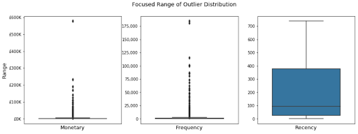
Figure 1 - The outliers plotted on a boxplot, showing the specific ranges of each variable and the areas on where to focus.
When visualising the data on a 3D projection, Figure 3, it is clear that removing the outliers from the dataset greatly helps focus more towards the bulk of the data. Furthermore, each variable was scaled, as Euclidean distance is sensitive to the scales or magnitude of the attributes, therefore the values would need standardising and brought into homogeneous ranges.
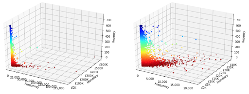
Figure 2 - The before and after the removals of outliers, displayed on a 3D projection.
Results

Figure 3 - 3D plotted dataset - colour coded for the different clusters.
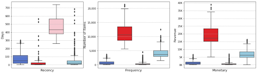
Figure 4 - Boxplot of the 3 variables broken down by the four clusters. Colours in the boxplot match the colours of the clusters in Figure 3.
From Figures 3 and 4, it is clear that cluster 1 would be classed as the ‘Best Customers’ due to significantly higher spend, much more than the other clusters. Additionally, the average frequency of purchases is higher and the recency of the latest purchase, on average, a lot lower.
Whilst cluster 2 appears to be the least valuable and more related to ‘Lost Customers’. The mean last purchase is over a year ago, with the frequency and monetary value of their purchases extremely low. However, it means that around a third of the consumer base show little signs of interaction.
Cluster 3 is considered the second best, as the recency remains low, however, the recency range of data points is the largest of all four clusters. The frequency and monetary values are relatively high.
Finally, cluster 0, it contains the most number of customers with 2,924. In Figure 10, cluster 0 sits on similar axes as cluster 2, however, the recency is significantly lower, supported in Figure 4. The recency range is the lowest, therefore the customers are still current, but the frequency and monetary averages remain low.